The goal of this document is to show typical codec�s analysis to support future tuning. x264 codec implementing H.264 standard was chosen as an example. Strong and weak spots of x264 in terms of encoding speed and video quality are found and recommendations on use of codec�s presets are given. This document may be of interest to companies analyzing usefulness of tuning/elaboration of their own codecs and also for users of x264 codec. More about YUVsoft�s services on developing, tuning and testing videocodecs and other R&D services and opportunities may be found at www.yuvsoft.com/technologies/codecs_testing/index.html.

Codec

We have chosen x264 as a demo codec because of few reasons. x264 has a lot of parameters for precise tuning, and many features of H.264 standard are implemented in it. Open sources of the codec allow a more detailed analysis of obtained testing results. Another reason is codec�s quality � according to H.264 comparisons[1], x264 is one of the best H.264 codecs for the present time.

We used a codec compiled from sources labeled as �x264-snapshot-20060406-2245�. The reference codec JM 9.8 was used for decoding.

Sequences

Sequence	Number of frames	Frames per second	Resolution and color space
1. foreman	300	30	352x288(YV12)
2. susi	374	25	704x576(YV12)
3. bbc	374	25	704x576(YV12)
4. battle	1599	24	704x288(YV12)
5. simpsons	365	24	720x480(YV12)
6. matrix	239	25	720x416(YV12)
7. mobile	372	25	704x576(YV12)

Our test set includes mainly movies and standard sequences from different sources with different types of motion. A more detailed description of all used sequences can be found in Appendix: Sequences Description.

Methodology

Averaging Methods and Explanation of Charts

One of the most important characteristics of a codec is quality of encoded video. Besides problems regarding how to measure �video quality�, there are difficulties in comparing different codecs or modes of functioning of a certain codec since it is non-trivial to represent quality by a single value. Some reasonable assumptions and well-grounded aggregation methods are necessary to perform such a comparison. The following approach was used.

First of all, we run all chosen presets of x264 for all test sequences at 10 different bitrates: 100, 225, 340, 460, 700, 938, 1140, 1340, 1840 and 2340 Kbps. Encoded sequences were compared with corresponding originals using objective metrics such as PSNR, SSIM, etc. It made us able to create and operate with Bitrate/Quality charts or Rate-Distortion curves of the codec. These data are necessary to correctly compare different modes (presets) of the codec, or, as it also might be the case, to correctly compare different codecs. We used the notion of �relative bitrate� meaning what bitrate in percents should be to achieve the same quality (by, for example, PSNR criterion) as for some reference preset whose bitrate is taken for 100%.

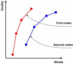
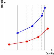
The first step to get relative bitrate of two presets (codecs) is �rotating� of Rate-Distortion (RD) charts, changing axis of the charts (Figure 1, Figure 2). It allows us to calculate ratio of bitrates for the same quality. The advantage of bitrates ratio for the same quality instead of, for example, PSNR difference for the same bitrate, is that bitrates ratio does not generally depend on an objective quality metric being used.

After that it is necessary to choose interval of averaging. We used an internal area of RD curves where missed bitrate values can be interpolates between the nearest values (see Figure 2). It means that we did not use extrapolation because of big possible mistakes of RD curves extrapolation. Linear interpolation was used to get values between the existing points. Previous experiments convinced us that more complex interpolation methods usually give very little for better accuracy.

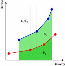
To get average values we calculated sizes of areas under the curves and divided one by the other (see Figure 3).


Figure 1. Source RD data	Figure 2. Axis rotation and interval choosing

Figure 3. Ratio of areas

To get relative encoding time for two presets, we calculated relative time for each sequence and use arithmetic mean to average those values. For each sequences we divided total encoding time for each preset (time to encode sequence with 10 bitrates) by encoding time of a chosen reference preset.

This method allows us to take into account small sequences with the same weight as long sequences.

Average Relative Bitrate graphs, which are often used in this document, are a visualization of relative speed and relative bitrate (for the same quality) for all presets. A certain default preset was selected as a reference; it is always placed in point (1, 1) on these figures. For each preset relative time and relative bitrate were calculated against the reference and placed on the charts as shown on Figure 4.

Figure 4. Speed (Encoding Time)/Quality chart example

Metrics Used in Comparison

During testing the following metrics were calculated:

� PSNR (Y component)

� SSIM (Y component)

� Blocking (Y component)

Information of these metrics can be found here:

http://www.compression.ru/video/quality_measure/info_en.html

All types of analysis in this document were made using Y-PSNR metric. Relative bitrates were calculated using this classic metric, as described in section �Averaging Methods and Explanation of Charts�.

Presets

We have chosen many different presets (codec parameters combinations) in order to try to select optimal presets in terms of speed and objective video quality.

Since we can�t test presets on all sequences available all over the world, so we compared presets on test sequences that were enumerated above. This test set is deemed to be representative for common applications.

The chosen presets are described in the following table. It might be convenient to print this table for a more convenient study of subsequent charts.

	Preset	Comments
1.	default	All parameters are set to their default values and the command line looks like: x264 ‑‑no-psnr ‑‑bitrate=<target_bitrate> ‑‑fps=<fps> -o <output> <input> <width>x<height> Other presets add additional parameters to this command line.
2.	-t 1	We want to see how trellis works in terms of speed/quality tradeoff. Trellis is a deletion of nonzero coefficients after DCT and quantization if it is among a group of zero coefficients. For example, if we have sequence 00001000 of quantized DCT coefficients, after trellis RDO optimization the only �one� can be zeroed.
3.	-t 2
4.	‑‑nr 5	Switches noise reduction on.
5.	‑‑no-fast-pskip	Disable early skip detection on P-frames.
6.	‑‑subme 1	Different modes of block partitioning and sub-pixel motion estimation. �‑‑subme 7� turns on optimal sub-block partitioning by encoding all partitions and choosing between them, so it works very long, but it can give quality comparable with multi-pass algorithms.
7.	‑‑subme 3
8.	‑‑subme 6
9.	‑‑subme 7
10.	‑‑me dia	Different motion estimation modes.
11.	‑‑me umh
12.	‑‑me esa
13.	‑‑subme 6 ‑‑b-rdo ‑b 3	RD-based mode decision for B-frames. We need to turn on subme=6 in order to make it works.
14.	‑‑no-chroma-me	Use only luma in motion estimation. It can improve speed, but if an image contains regions that have the same luma component, but different colors (�Mobile� sequence has such regions), motion estimation will fail.
15.	‑‑weightb -b 3
16.	-b 3 ‑‑b-bias 5 ‑‑b-pyramid ‑‑weightb ‑‑b-rdo ‑‑subme 6 ‑‑bime
17.	‑‑direct none	Several motion vector prediction modes.
18.	‑‑direct spatial
19.	‑‑direct temporal
20.	‑‑direct auto
21.	‑‑analyse=none	Different modes of MB partitioning.
22.	‑‑analyse=all -8	Different modes of MB partitioning.
23.	‑‑pass 1 ‑‑pass 2	Multipass algorithms. They give better quality, but work two and three times slower, respectively.
24.	‑‑pass 1 ‑‑pass 3 ‑‑pass 2
25.	‑‑ratetol 0.1	Test how quality and speed would change, if the codec has to keep target bitrate more precisely.
26.	‑‑nf	Disable loop filter (turn off deblocking).
27.	‑‑no-cabac	Use CAVLC (variable length codes) instead of CABAC (arithmetic compression).
28.	‑‑ref 10	Use greater number of reference frames. Can significantly improve motion compensation accuracy.
29.	‑‑scenecut 10	Insert extra I-frames more aggressively.
30.	‑‑me=umh ‑‑merange=32 ‑‑subme=6 ‑‑ref=16 ‑‑analyse=all ‑‑direct=spatial ‑‑pbratio=1.5 ‑‑bframes=3 ‑‑weightb ‑‑pass=1 ‑‑me=umh ‑‑merange=32 ‑‑subme=6 ‑‑ref=16 ‑‑analyse=all< br> ‑‑direct=spatial ‑‑pbratio=1.5 ‑‑bframes=3 ‑‑weightb ‑‑pass=2	Encode with the best possible quality available.
31.	‑‑me=dia ‑‑merange=16 ‑‑subme=1 ‑‑analyse=none ‑‑direct=spatial ‑‑pbratio=1.5 ‑‑bframes=1	Here we take the previous preset () and decrease parameter values in order to reach good quality with better speed.
32.	‑‑no-b-adapt ‑‑no-cabac ‑‑analyse=p8x8 ‑‑me dia ‑‑subme=1 ‑‑no-chroma-me
33.	-b 4 ‑‑b-pyramid -r 16 ‑‑analyse=all ‑‑direct auto ‑‑weightb ‑‑me umh ‑‑subme=7 ‑‑b-rdo ‑‑bime -8 ‑‑pass=1 -b 4 ‑‑b-pyramid -r 16 ‑‑analyse=all ‑‑direct auto ‑‑weightb ‑‑me umh ‑‑subme=7 ‑‑b-rdo ‑‑bime -8 ‑‑pass=2
34.	‑‑me=umh ‑‑merange=32 ‑‑subme=6 ‑‑ref=16 ‑‑analyse=all ‑‑direct=spatial ‑‑pbratio=1.5 ‑‑bframes=3 ‑‑weightb
35.	‑‑me=umh ‑‑merange=16 ‑‑subme=6 ‑‑ref=8 ‑‑analyse=all ‑‑direct=spatial ‑‑pbratio=1.5 ‑‑bframes=3
36.	‑‑me=umh ‑‑merange=16 ‑‑ref=4 ‑‑analyse=all ‑‑direct=spatial ‑‑pbratio=1.5 ‑‑bframes=3 ‑‑weightb
37.	-b 3 ‑‑b-bias 5 ‑‑b-pyramid ‑‑weightb ‑‑b-rdo ‑‑bime ‑‑subme 7 -8 ‑‑ref 4
38.	‑‑subme 7 ‑‑ref 10	We want to evaluate relative influence of partitioning, motion compensation and trellis parameters.
39.	‑‑subme 7 -t 1
40.	‑‑ref 10 -t 1
41.	-b 3 ‑‑b-bias 5 ‑‑b-pyramid ‑‑weightb ‑‑b-rdo ‑‑bime -8 -t 1	Some other variants of good quality presets.
42.	‑‑subme 6 -b 5 ‑‑b-bias 5 ‑‑b-pyramid
43.	-b 4 ‑‑b-pyramid -r 10 ‑‑analyse=all ‑‑direct auto ‑‑weightb ‑‑me umh ‑‑subme=7 ‑‑b-rdo ‑‑bime -8 -t 1
44.	-b 4 ‑‑b-pyramid -r 10 ‑‑direct auto ‑‑weightb ‑‑me umh ‑‑subme=7 ‑‑b-rdo ‑‑bime -8
45.	-b 3 ‑‑b-bias 5 ‑‑b-pyramid ‑‑weightb ‑‑b-rdo ‑‑subme=6 ‑‑bime ‑‑pass 1 -b 3 ‑‑b-bias 5 ‑‑b-pyramid ‑‑weightb ‑‑b-rdo ‑‑subme=6 ‑‑bime ‑‑pass 2
46.	-b 4 ‑‑b-pyramid -r 8 ‑‑analyse=all ‑‑direct auto ‑‑weightb ‑‑me umh ‑‑subme 7 ‑‑b-rdo ‑‑bime -8 ‑‑pass 1 -b 4 ‑‑b-pyramid -r 8 ‑‑analyse=all ‑‑direct auto ‑‑weightb ‑‑me umh ‑‑subme 7 ‑‑b-rdo ‑‑bime -8 ‑‑pass 2
47.	-b 3 ‑‑b-bias 5 ‑‑b-pyramid ‑‑weightb ‑‑subme 7 -8 -ref 4
48.	-b 4 ‑‑b-pyramid -r 8 ‑‑analyse=all ‑‑direct auto ‑‑weightb ‑‑me umh -8 ‑‑pass 1 -b 4 ‑‑b-pyramid -r 8 ‑‑analyse=all ‑‑direct auto ‑‑weightb ‑‑me umh -8 ‑‑pass 2

Presets Measurements Results

First of all, it should be once again mentioned that in this comparison we are interested only in average objective quality vs. encoding speed tradeoff. So, all conclusions (�better�, �worse�, �faster�, etc.) will be made from this point of view. Of course, there are lots of other codec�s parameters, which are not considered here (bitrate keeping, bitrate variations, etc.)

Sometimes phrases like �preset�s quality is better by N%� are used in this comparison. Such phrases should be understood as �preset requires N% less bitrate to encode given sequences with the same objective quality�.

We name a preset �sub-optimal� if there is no other preset which gives better quality and works faster on given sequences. In other words, its dot is not covered by any other dots on a speed/quality chart. A number of sub-optimal presets can be selected for the same sequences.

In the following charts there are results of presets measurements for test sequences. On horizontal axis there is relative encoding time ‑ how long a given preset works relative to the default preset. And on vertical axis there is relative bitrate. This value depicts encoded sequence size for the same quality comparing to the default preset. The default preset has value (1, 1).

A more detailed description can be found in section �Averaging Methods and Explanation of Charts�.

Charts of Quality/Speed tradeoff are shown for each sequence on Figure 5 - Figure 18 below. We have made several charts showing certain zoomed regions in order to simplify presets comparison.

Figure 5. Speed/Quality tradeoff of all presets on �Foreman� sequence

Figure 6. Speed/Quality tradeoff of all presets on �Foreman� sequence, zoomed region

Figure 7. Speed/Quality tradeoff of all presets on �Susi� sequence

Figure 8. Speed/Quality tradeoff of all presets on �Susi� sequence, zoomed region

Figure 9. Speed/Quality tradeoff of all presets on �BBC� sequence

Figure 10. Speed/Quality tradeoff of all presets on �BBC� sequence, zoomed region

Figure 11. Speed/Quality tradeoff of all presets on �Battle� sequence

Figure 12. Speed/Quality tradeoff of all presets on �Battle� sequence, zoomed region

Figure 13. Speed/Quality tradeoff of all presets on �Simpsons� sequence

Figure 14. Speed/Quality tradeoff of all presets on �Simpsons� sequence, zoomed region

Figure 15. Speed/Quality tradeoff of all presets on �Matrix� sequence

Figure 16. Speed/Quality tradeoff of all presets on �Matrix� sequence, zoomed region

Figure 17. Speed/Quality tradeoff of all presets on �Mobile� sequence

Figure 18. Speed/Quality tradeoff of all presets on �Mobile� sequence, zoomed region

Figure 19 and Figure 20 show averaged results for all test set. Geometric mean was used for bitrate and arithmetic mean for speed calculation.

Of course, in some cases charts for separate sequences differ rather strongly and it is not quite correct to average out all charts. But averaged data help to understand the situation for the entire test set and to analyze results easier.

Figure 21 shows quality/speed for only sub-optimal presets for the entire test set. All others preset were deleted.

Figure 19. Speed/Quality tradeoff of all presets for the entire test set

Figure 20. Speed/Quality tradeoff of all presets for the entire test set, zoomed region

Figure 21. Speed/Quality tradeoff of only sub-optimal presets for the entire test set

Simple Presets Analysis

Here we analyze �simple� presets ‑ presets that differ from the default one by turning on one (in most cases) codec�s parameter.

	Preset	Comments
2.	-t 1	Trellis 1 makes small quality improvement (4%) with moderate speed decrease (16%). On average there are a number of presets which are better than trellis optimization (variations of �‑‑direct� presets, , ). On the other hand, this preset is not covered by any other preset on sequences �Matrix�, �Simpsons�, �Battle� and �BBC�.
3.	-t 2	Trellis 2 further improves quality (~6.5% comparing to default preset), but works much longer (2.3 times). Many other presets cover this preset both by quality and speed (for all sequences). Probably, usage of this preset is not optimal from the speed/quality tradeoff point of view.
4.	‑‑nr 5	Noise reduction does not give significant quality change for our test set. Encoding speed increased only by 2%. Usage of this preset does not lead to any significant changes of quality by objective metrics.
5.	‑‑no-fast-pskip	On average, this preset is worse than the default one (+21% of encoding time with approximately the same quality). This preset gives maximum quality improvements on �Matrix� sequence. Usage of this preset for encoding is rather dubious.
6.	‑‑subme 1	�‑‑subme� parameter is a useful tool to vary quality/speed tradeoff. �‑‑subme 1� is one of the fastest presets in our comparison. It requires only 45% of default preset time for encoding and 9% of additional bitrate for the same quality. This preset is sub-optimal for all sequences except �Mobile� (complex �preset is better there) �‑‑subme 3� decreases encoding speed by 30% and saves 2% of bitrate. This preset is sub-optimal for all sequences except �Mobile� too. �‑‑subme 6� and �‑‑subme 7� options are not sub-optimal, they are covered by many others presets. Probably, it is reasonable to use values �1� or �3� to increase encoding speed. Values �6� and �7� don�t lead to optimal encoding.
7.	‑‑subme 3
8.	‑‑subme 6
9.	‑‑subme 7
10.	‑‑me dia	DIA algorithm works a little faster (only app. 3.5%) than the default one and gives approximately the same quality. In fact, this ME method doesn�t differ much comparing to HEX (default) by speed/quality tradeoff criterion. UMH works 20% slower and saves only 2% of bitrate. It is not sub-optimal for all sequences except �Simpsons� and �BBC�. Speed/quality tradeoff for ME ESA is not very good. Lots of other presets can produce smaller sequences with the same quality and do it faster.
11.	‑‑me umh
12.	‑‑me esa
13.	‑‑subme 6 ‑‑b-rdo ‑b 3	Works 1.5 times longer than the default preset, saves 8% of bitrate. This preset is not sub-optimal for all sequences. The reason of that, probably, that not all possibilities of B-frames usage are exploited in this preset.
14.	‑‑no-chroma-me	This preset works 19% faster than the default one. Differences in quality for luma (Y) plane are not significant, in U and V planes it is 3.5% worse than the default preset.
15.	‑‑weightb -b 3	This preset is better than the default one (5% faster, saves 4% of bitrate) on average. But results are varying strongly from sequence to sequence. Best results are attained on �Foreman�, �Susi� and �Mobile� sequences, on �BBC� sequence this preset is worse than default, on other sequences differences are not significant. Results of this preset are very close to �‑‑direct� options variations.
16.	-b 3 ‑‑b-bias 5 ‑‑b‑pyramid ‑‑weightb ‑‑b-rdo ‑‑subme 6 ‑‑bime	On all sequences it works very similar to �preset (little better and slower).
17.	‑‑direct none	On average all values except �none� works better (~5% of bitrate) and with the same speed as the default one. But results strongly depend on a sequence. On �Foreman�, �Susi� and �Mobile�, these �spatial�, �temporal� and �auto� presets show better quality (10-15% of bitrate saving) while being not slower than the default preset. On �Battle�, �Simpsons� and �Matrix� sequences differences are not significant. On �BBC� sequence all presets are worse than the default one, but the differences varies strongly (see Figure 9, Figure 10). �none� value always leads to both quality and speed decrease. Probably, this option is not optimal.
18.	‑‑direct spatial
19.	‑‑direct temporal
20.	‑‑direct auto
21.	‑‑analyse=none	This preset works rather fast on average (64% of default preset encoding time), but increases bitrate 8% for the same quality. Preset is sub-optimal at most sequences.
22.	‑‑analyse=all -8	Slower (6%) and a little better (3%) than the default preset on average. This preset is sub-optimal on �Matrix�, �Simpsons� and �Battle� sequences. On other sequences this preset is covered by �‑‑direct� option presets.
23.	‑‑pass 1 ‑‑pass 2	2-pass encoding is really almost 2 times faster than the 1-pass default preset. It saves 7% of bitrate for the same quality. This preset is sub-optimal on �BBC� and �Matrix� sequences only. 2-pass encoding is not always optimal in terms of speed/quality tradeoff.
24.	‑‑pass 1 ‑‑pass 3 ‑‑pass 2	Encoding time linearly grows with increase of number of passes. But quality increasing is not significant comparing to 2-pass encoding (+0.6% of bitrate). This preset is not sub-optimal for all sequence.
25.	‑‑ratetol 0.1	Increasing restrictions on rate variation, we decrease resulting quality of video sequence (+5% of bitrate on average). Speed of this preset is very near to the default one.
26.	‑‑nf	Turning off loop filter results in quality degradation (7% of bitrate for the same quality) and small speed increase (5%). Preset is always not sub-optimal. Probably, user should have serious reasons to turn off deblocking filter.
27.	‑‑no-cabac	It is interesting to note that using CALVC instead of CABAC increases speed by 7% only. But quality degrades significantly (12% on average). Probably, implementation of CALVC in x264 is not very good now.
28.	‑‑ref 10	Using 10 frames instead of 1 in the default preset increases encoding time to 65% and saves 7% on average. But this preset is not sub-optimal for all sequences except �Simpsons� and �BBC�. For example, B-usage in most cases is better than 10 reference frames.
29.	‑‑scenecut 10	The difference between this preset and the default one is very small for all sequences.

Summary:

� Best options by speed/quality tradeoff criterion:

o �‑‑direct� options (all except �none� value)

o �-subme 3� or �-subme 1�

o �‑‑weightb� (use with B frames)

� Trellis usage really increases quality of encoded sequence, but this feature requires considerably bigger encoding time

� �-subme 6� or �-subme 7� are implementations of interesting RC ideas, but they are not optimal as standalone options

� �‑‑no-fast-pskip� is a rather strange option. It increases encoding time, but does not lead to quality improvement on average

� ME algorithm changes allow to alter speed/quality tradeoff, but they are not optimal as standalone options. Differences between DIA and HEX are not significant, ESA works too long.

� �‑‑analyse=none� option is a rather good option to speed up encoding process.

� �‑‑direct� option is a very powerful option, but it does not always work. Sometimes it can even decrease encoding quality

Complex Presets Analysis

There are a number of rather complex presets differing a lot from default. That is why it is reasonable to describe them separately.

	Preset	Comments
30.	‑‑me=umh ‑‑merange=32 ‑‑subme=6 ‑‑ref=16 ‑‑analyse=all ‑‑direct=spatial ‑‑pbratio=1.5 ‑‑bframes=3 ‑‑weightb ‑‑pass=1 ‑‑me=umh ‑‑merange=32 ‑‑subme=6 ‑‑ref=16 ‑‑analyse=all ‑‑direct=spatial ‑‑pbratio=1.5 ‑‑bframes=3 ‑‑weightb ‑‑pass=2	This preset is not sub-optimal on average. It works 8 times longer than default preset and saves 22% of bitrate, but preset 46() is faster and produce better quality for most sequences.
31.	‑‑me=dia ‑‑merange=16 ‑‑subme=1 ‑‑analyse=none ‑‑direct=spatial ‑‑pbratio=1.5 ‑‑bframes=1	This is a high speed preset. It works two times faster than default one, and requires 14% more bitrate for the same quality. This preset is sub-optimal for most sequences.
32.	‑‑no-b-adapt ‑‑no-cabac ‑‑analyse=p8x8 ‑‑me dia ‑‑subme=1 ‑‑no-chroma-me	This preset is the fastest in our comparison (42.6% of default preset speed). Unfortunately, it has problems with quality � it requites 29% more bitrate for the same quality.
33.	-b 4 ‑‑b-pyramid -r 16 ‑‑analyse=all ‑‑direct auto ‑‑weightb ‑‑me umh ‑‑subme=7 ‑‑b-rdo ‑‑bime -8 ‑‑pass=1 -b 4 ‑‑b-pyramid -r 16 ‑‑analyse=all ‑‑direct auto ‑‑weightb ‑‑me umh ‑‑subme=7 ‑‑b-rdo ‑‑bime -8 ‑‑pass=2	The slowest preset in our comparison. Increased number of reference frames, comparing to �preset, does not improve quality (very small improvement on �Foreman� and �Mobile� sequences with relatively slow motion). This preset works approximately 9.3 times slower than the default one, saving 28% of bitrate.
34.	‑‑me=umh ‑‑merange=32 ‑‑subme=6 ‑‑ref=16 ‑‑analyse=all ‑‑direct=spatial ‑‑pbratio=1.5 ‑‑bframes=3 ‑‑weightb	This preset is not effective for most sequences in our test.
35.	‑‑me=umh ‑‑merange=16 ‑‑subme=6 ‑‑ref=8 ‑‑analyse=all ‑‑direct=spatial ‑‑pbratio=1.5 ‑‑bframes=3	This preset works with approximately the same quality as , but 1.5-2 times faster. So decreasing �merange� from 32 to 16 and ref from 16 to 8 does not decrease quality notably.
36.	‑‑me=umh ‑‑merange=16 ‑‑ref=4 ‑‑analyse=all ‑‑direct=spatial ‑‑pbratio=1.5 ‑‑bframes=3 ‑‑weightb	Measurement results of these presets greatly depend on sequence type. On some sequences one of these presets is optimal and on the other sequences they are covered by many other presets.
37.	-b 3 ‑‑b-bias 5 ‑‑b-pyramid ‑‑weightb ‑‑b-rdo ‑‑bime ‑‑subme 7 -8 ‑‑ref 4
38.	‑‑subme 7 ‑‑ref 10	There are reasons to think that ‑‑subme 7 is not the optimal choice in almost all situations.
39.	‑‑subme 7 -t 1
40.	‑‑ref 10 -t 1
41.	-b 3 ‑‑b-bias 5 ‑‑b-pyramid ‑‑weightb ‑‑b-rdo ‑‑bime -8 -t 1	This preset works slower than �1.5 times, but gives better quality (~20%)
42.	‑‑subme 6 -b 5 ‑‑b-bias 5 ‑‑b-pyramid	It is not sub-optimal on almost every sequence (except �Foreman� and �Susi�). On �Foreman� sequence it works faster, than the default preset.
43.	-b 4 ‑‑b-pyramid -r 10 ‑‑analyse=all ‑‑direct auto ‑‑weightb ‑‑me umh ‑‑subme=7 ‑‑b-rdo ‑‑bime -8 -t 1	This preset works very similar to �preset. Turning on options �‑‑analyse=all -t 1� doesn�t improve quality on every sequence
44.	-b 4 ‑‑b-pyramid -r 10 ‑‑direct auto ‑‑weightb ‑‑me umh ‑‑subme=7 ‑‑b-rdo ‑‑bime -8	This preset is rather balanced on our test suite. Working 3.5 times slower than the default one, it saves 22% of bitrate for the same quality.
45.	-b 3 ‑‑b-bias 5 ‑‑b-pyramid ‑‑weightb ‑‑b-rdo ‑‑subme=6 ‑‑bime ‑‑pass 1 -b 3 ‑‑b-bias 5 ‑‑b-pyramid ‑‑weightb ‑‑b-rdo ‑‑subme=6 ‑‑bime ‑‑pass 2	This preset is not sub-optimal on all sequences, except �Mobile�. But it works pretty fast for its quality (3 times longer than the default one).
46.	-b 4 ‑‑b-pyramid -r 8 ‑‑analyse=all ‑‑direct auto ‑‑weightb ‑‑me umh ‑‑subme 7 ‑‑b-rdo ‑‑bime -8 ‑‑pass 1 -b 4 ‑‑b-pyramid -r 8 ‑‑analyse=all ‑‑direct auto ‑‑weightb ‑‑me umh ‑‑subme 7 ‑‑b-rdo ‑‑bime -8 ‑‑pass 2	Probably, it is the best preset for high quality encoding among all tested. It gives 20-40% bitrate saving (28% on average) increasing time of encoding approximately 7 times.
47.	-b 3 ‑‑b-bias 5 ‑‑b-pyramid ‑‑weightb ‑‑subme 7 -8 -ref 4	It is sub-optimal on many sequences (�Foreman�, �Susi�, �Battle�, �Simpsons� and �Matrix�). On �BBC� and �Mobile� it is covered by only one preset (by �on �BBC� and by �on �Mobile�)
48.	-b 4 ‑‑b-pyramid -r 8 ‑‑analyse all ‑‑direct auto ‑‑weightb ‑‑me umh -8 ‑‑pass 1 -b 4 ‑‑b-pyramid -r 8 ‑‑analyse all ‑‑direct auto ‑‑weightb ‑‑me umh -8 ‑‑pass 2	This preset is less effective than �on all sequences but �Mobile�.

Summary:

� Complex presets of x264 allow to achieve high quality or high speed

� Combinations of different options comparing to a single codec option modification (as in simple presets) further improve speed/quality tradeoff

� Usage of options dealing with B-frames optimization is a good way to achieve the perfect speed/quality tradeoff in the area of moderate encoding complexity

Conclusions

� Acquired results show that settings of x264 really can control codec�s quality/speed tradeoff with great flexibility. Speed of the codec can be varied more than 20 times, producing streams with sizes differing up to 50% from each other for the same quality.

� The default preset is not sub-optimal for our test set, but its speed/quality tradeoff is good enough.

� Not all implemented features of x264 lead to speed/quality tradeoff improvements. One of the possible reasons of that fact can be inefficient implementation of certain features.

� It can be suggested that the following presets should be additionally tuned to improve speed/quality tradeoff:

o ‑‑subme 6 and 7

o trellis based RDO optimization (�-t� option)

o ‑‑direct options works great but not for all sequences; probably, this feature should be turned on adaptively

o multi-pass encoding and ESA ME (they work too slow)

o CAVLC encoding

� We can propose the following settings to use as different x264 presets for various applications and purposes:

Preset name	Settings
Fastest	‑‑me=dia ‑‑merange=16 ‑‑subme=1 ‑‑analyse=none ‑‑direct=spatial ‑‑pbratio=1.5 ‑‑bframes=1
Fast	‑‑subme=1
Tradeoff	‑‑subme=3
Good	-b 3 ‑‑b-bias 5 ‑‑b-pyramid ‑‑weightb ‑‑b-rdo ‑‑bime -8 -t 1
Best	-b 4 ‑‑b-pyramid -r 10 ‑‑analyse=all ‑‑direct auto ‑‑weightb ‑‑me umh ‑‑subme=7 ‑‑b-rdo ‑‑bime -8 -t 1
Extra Quality	-b 4 ‑‑b-pyramid -r 8 ‑‑analyse=all‑‑direct auto ‑‑weightb ‑‑me umh ‑‑subme 7 ‑‑b-rdo ‑‑bime -8 ‑‑pass 1 -b 4 ‑‑b-pyramid -r 8 ‑‑analyse=all ‑‑direct auto ‑‑weightb ‑‑me umh ‑‑subme 7 ‑‑b-rdo ‑‑bime -8 ‑‑pass 2

The table below shows relative speed and relative bitrate for the same quality for proposed presets comparing to the default one.

Preset Name	Speed, %	Average bitrate, %
Fastest	47	114
Fast	56	109
Tradeoff	70	102
Good	121	89
Best	369	77
Extra Quality	710	72

Appendix: Sequences Description

Foreman

Sequence title	Foreman
Resolution	352x288
Number of frames	300
Color space	YV12
Frames per second	30
Source	Uncompressed (standard sequence), progressive

Figure 22. Frame 77 of �Foreman�

Figure 23. Frame 258 of �Foreman�

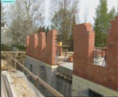
This is one of the most famous sequences. It represents a face with very rich mimic. Motion is not very intensive here, but on the other hand it is disordered, not straightforward. Intricate character of motion may create problems for the motion compensation process. In addition camera is shaking, that makes the image unsteady. In the end of the sequence camera suddenly turns to the building site and there follows an almost motionless scene. So this sequence also shows codec�s behavior on a static scene after intensive motion.

Susi

Sequence title	Susi
Resolution	704x576
Number of frames	374
Color space	YV12
Frames per second	25
Source	MPEG-2 (40Mbit), Smart Deinterlace

Figure 24. Frame 193 of �Susi�

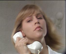
This sequence is characterized by high-level noise and slow motion. In its first part the scene is almost static (the girl only blinks), then there is some motion (she abruptly moves her head) and then the scene becomes almost static again. Noise is suppressed on every second frame due to B-frames usage in a MPEG-2 codec.

BBC

Sequence title	BBC
Resolution	704x576
Number of frames	374
Color space	YV12
Frames per second	25
Source	Uncompressed (standard sequence), Smart Deinterlace


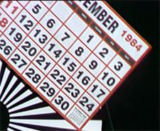
Figure 25. Frame 185 of �BBC�	Figure 26. Frame 258 of �BBC�

This sequence is characterized by pronounced rotary motion which is quite uncommon for typical video and, therefore, can be used as a crash-test for motion estimation and other algorithms. The sequence contains a rotating striped drum with different pictures and photos on it. Quality of the compressed sequence can be evaluated by observing details on these images.

Battle

Sequence title	Battle
Resolution	704x288
Number of frames	1599
Color space	YV12
Frames per second	24
Source	MPEG-2 (DVD), FlaskMPEG deinterlace

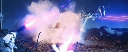
Figure 27. Frame 839 of �Battle�

This sequence is a fragment of the �Terminator-2� movie and represents its very beginning. In terms of compression this sequence is the most difficult one among all other sequences that took part in the comparison. That is because of three main reasons: constant brightness changes (explosions and laser flashes, see the picture above), relatively very quick motion and frequent changes of the scene that make codecs often compress frames as I-frames.

Simpsons

Sequence title	Simpsons
Resolution	720x480
Number of frames	365
Color space	YV12
Frames per second	24
Source	MPEG-2 (DVD), progressive

Figure 28. Frame 50 of �Simpsons�

This sequence is a fragment of �Simpsons� cartoon film. This is a classic representative of cartoon films: sketchy movement, great number of monochrome regions with abrupt edges between them. Previously this sequence was compressed in MPEG-2 with rather low bitrate giving notable compression artifacts.

Matrix

Sequence title	Matrix
Resolution	720x416
Number of frames	239
Color space	YV12
Frames per second	25
Source	MPEG-2 (DVD), Smart Deinterlace

Figure 29. Frame 226 of �Matrix�

This sequence is a fragment of �Matrix� movie. Relatively simple movement and quite dim colors allows codecs to treat this sequence in rather simple way.

Mobile

Sequence title	mobile
Resolution	704x576
Number of frames	372
Color space	YV12
Frames per second	25
Source	Uncompressed (standard sequence), Smart Deinterlace

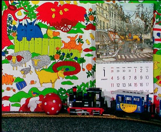
Figure 30. Frame 100 of �Mobile�

This sequence contains relatively slow, but complicated motion. There are parts of the picture that move in opposite directions, and this situation may be rather complex for motion estimation algorithms. Also there are parts of the picture that have the same brightness, but different color components.